Likelihood-free inference

Often the likelihood \(p(x \mid \theta)\) cannot be written down, but data can be simulated for any \(\theta\). Likelihood-free (simulation-based) inference works with the simulator alone. This notebook compares three methods from psiphy.sbi on a problem whose exact posterior is known:

1. Rejection ABC (rABC): keep prior draws whose simulation lands close to the data. Simple, but needs many simulations.

2. BOLFI (BOLFI): learn a Gaussian-process model of the discrepancy with Bayesian optimisation, then sample the resulting synthetic likelihood with any psiphy sampler. Typically needs orders of magnitude fewer simulations — what matters when each simulation is expensive.

3. LFIRE (LFIRE): estimate the likelihood-to-evidence ratio \(p(x \mid \theta)/p(x)\) with a classifier. No distance or tolerance to tune; the classifier learns how to weigh the summaries.

Contents: the problem → exact reference → rejection ABC → BOLFI → LFIRE → acquisition functions and batch proposals → saving/resuming.

import os
import tempfile

import numpy as np
import matplotlib.pyplot as plt

from psiphy.sbi.bolfi import BOLFI
from psiphy.sbi.rejection_abc import rABC
from psiphy.mcmc import MHSampler
from psiphy.utils.prior import UniformPrior
from psiphy.toy_models import GaussianSignal

np.random.seed(3)

---

1 Problem and discrepancy

Data: \(N = 50\) draws from \(\mathcal{N}(\mu, \sigma^2)\); unknowns \(\theta = (\mu, \sigma)\). We pretend we can only simulate.

Both methods compare simulated and observed data through summary statistics — here the sample mean \(\bar{x}\) and standard deviation \(s\) — combined into a discrepancy scaled by their expected sampling variances (\(\mathrm{Var}\,\bar{x} \approx s^2/N\), \(\mathrm{Var}\,s \approx s^2/2N\)):

\[d(\theta) = N\left[\frac{(\bar{x}_\theta - \bar{x}_{\rm obs})^2}{s_{\rm obs}^2} + \frac{2\,(s_\theta - s_{\rm obs})^2}{s_{\rm obs}^2}\right]\]

With this scaling \(d\) behaves like a \(\chi^2\), which BOLFI’s default 'exp' kernel (\(\mathcal{L} \propto e^{-d/2}\)) assumes.

gs = GaussianSignal(N=50)
theta_true = np.array([1.5, 0.8])
x_obs = gs.simulate(theta_true)

N = len(x_obs)
m_obs, s_obs = x_obs.mean(), x_obs.std(ddof=1)

def discrepancy(x_sim):
    return N * ((x_sim.mean() - m_obs) ** 2 / s_obs**2 + 2 * (x_sim.std(ddof=1) - s_obs) ** 2 / s_obs**2)

prior = UniformPrior({'mu': (0, 3), 'sigma': (0.1, 2.5)})
labels = [r'$\mu$', r'$\sigma$']
print(f'observed: mean = {m_obs:.3f}, std = {s_obs:.3f}')

observed: mean = 1.265, std = 0.807

---

2 Exact reference posterior

Because this toy model has a known likelihood, we can get the exact posterior with MCMC and use it to judge the likelihood-free results.

def log_post_exact(t):
    lp = prior.log_prob(t)
    return lp + gs.log_prob(t, x_obs) if np.isfinite(lp) else -np.inf

exact = MHSampler(log_post_exact, n_walkers=32).run(prior.sample(32), n_steps=3000)
s_exact = exact.get_chain(flat=True, discard='auto', thin=5)
print('exact mean:', s_exact.mean(0).round(3), '  std:', s_exact.std(0).round(3))

exact mean: [1.267 0.829]   std: [0.119 0.086]

---

3 Rejection ABC

Draw \(\theta\) from the prior, simulate, keep \(\theta\) if \(d < \varepsilon\). Smaller \(\varepsilon\) is more accurate but accepts fewer draws.

n_sims_abc = 30000
abc = rABC(
    simulator=lambda t: gs.simulate(t),
    distance=lambda x_o, x_s: discrepancy(x_s),
    observation=x_obs,
    prior={'mu': None, 'sigma': None},
    bounds={'mu': (0, 3), 'sigma': (0.1, 2.5)},
    N=n_sims_abc, eps=2.0, verbose=False,
)
abc.run()
s_abc = np.array(abc.accepted_param)
print(f'accepted {len(s_abc)} / {n_sims_abc} ({100 * len(s_abc) / n_sims_abc:.1f}%)')
print('ABC mean:', s_abc.mean(0).round(3), '  std:', s_abc.std(0).round(3))

accepted 227 / 30000 (0.8%)
ABC mean: [1.253 0.834]   std: [0.147 0.095]

---

4 BOLFI

1. learn_likelihood evaluates \(d(\theta)\) at a Latin-hypercube initial design, then repeatedly fits a GP to all evaluations and simulates where the acquisition function points (default: lower confidence bound, which balances low predicted \(d\) against GP uncertainty).

2. The GP mean \(\hat d(\theta)\) gives a synthetic log-likelihood \(-\hat d/2\).

3. sample_posterior samples it with MHSampler, NestedSampler, importance sampling or SMC.

The distance argument is a function of \(\theta\) that runs the simulator and returns \(d\).

bolfi = BOLFI(lambda t: discrepancy(gs.simulate(t)), prior, acquisition='LCB', verbose=False)
bolfi.learn_likelihood(n_calls=100, random_state=0)

s_bolfi = bolfi.sample_posterior(5000, method='MCMC', n_walkers=32, n_burn=500)
print(f'simulations used: {len(bolfi.y)}')
print('BOLFI mean:', s_bolfi.mean(0).round(3), '  std:', s_bolfi.std(0).round(3))

simulations used: 100
BOLFI mean: [1.229 0.838]   std: [0.081 0.126]

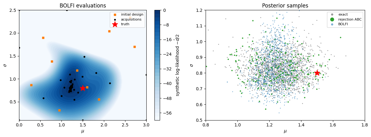
Where did BOLFI simulate? The points cluster in the high-likelihood region; the GP surrogate of the synthetic log-likelihood is shown in the background.

mu_g, sg_g = np.meshgrid(np.linspace(0, 3, 120), np.linspace(0.1, 2.5, 120))
grid = np.column_stack([mu_g.ravel(), sg_g.ravel()])
loglike_grid = bolfi.log_likelihood(grid).reshape(mu_g.shape)

fig, axes = plt.subplots(1, 2, figsize=(12, 4.5))
ax = axes[0]
cf = ax.contourf(mu_g, sg_g, np.maximum(loglike_grid, -60), levels=30, cmap='Blues')
plt.colorbar(cf, ax=ax, label=r'synthetic log-likelihood $-\hat d/2$')
ax.scatter(*bolfi.X[:10].T, c='C1', s=18, marker='s', label='initial design')
ax.scatter(*bolfi.X[10:].T, c='k', s=10, label='acquisitions')
ax.plot(*theta_true, 'r*', ms=14, label='truth')
ax.set(xlabel=labels[0], ylabel=labels[1], title='BOLFI evaluations')
ax.legend(fontsize=8, loc='upper right')

ax = axes[1]
ax.plot(*s_exact[::10].T, '.', c='0.6', ms=2, label='exact')
ax.plot(*s_abc.T, '.', c='C2', ms=4, label='rejection ABC')
ax.plot(*s_bolfi[::5].T, '.', c='C0', ms=2, alpha=0.5, label='BOLFI')
ax.plot(*theta_true, 'r*', ms=14)
ax.set(xlabel=labels[0], ylabel=labels[1], xlim=(0.8, 1.8), ylim=(0.5, 1.2), title='Posterior samples')
ax.legend(fontsize=8, markerscale=4)
plt.tight_layout()
plt.show()

fig, axes = plt.subplots(1, 2, figsize=(11, 3.5))
for i, ax in enumerate(axes):
    rng = (s_exact[:, i].min(), s_exact[:, i].max())
    ax.hist(s_exact[:, i], bins=40, range=rng, density=True, histtype='step', color='k', lw=1.5, label='exact')
    ax.hist(s_abc[:, i], bins=20, range=rng, density=True, alpha=0.4, color='C2', label='rejection ABC')
    ax.hist(s_bolfi[:, i], bins=40, range=rng, density=True, alpha=0.4, color='C0', label='BOLFI')
    ax.axvline(theta_true[i], c='r', lw=1)
    ax.set_xlabel(labels[i])
axes[0].legend(fontsize=8)
plt.tight_layout()
plt.show()

print(f"{'method':15s} {'simulations':>12s}   mean (mu, sigma)    std (mu, sigma)")
for name, s, n in [('exact', s_exact, '—'), ('rejection ABC', s_abc, n_sims_abc), ('BOLFI', s_bolfi, len(bolfi.y))]:
    print(f"{name:15s} {str(n):>12s}   {np.round(s.mean(0), 3)}   {np.round(s.std(0), 3)}")

method           simulations   mean (mu, sigma)    std (mu, sigma)
exact                      —   [1.267 0.829]   [0.119 0.086]
rejection ABC          30000   [1.253 0.834]   [0.147 0.095]
BOLFI                    100   [1.229 0.838]   [0.081 0.126]

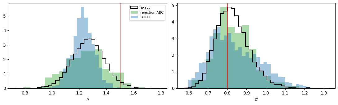
Why is every posterior, including the exact one, below the true :math:`mu`? The 50 observed values have a sample mean about two standard errors below the true mean (printed below). All methods correctly follow the data there; the comparison that matters is with the exact posterior, not with the true value. Calibration over many data sets is shown in Section 7 of the Importance sampling and SMC tutorial.

se = s_obs / np.sqrt(N)
print(f'sample mean = {m_obs:.3f}, true mean = {theta_true[0]}, standard error = {se:.3f}'
      f'  ->  data offset = {(m_obs - theta_true[0]) / se:+.1f} sigma')

sample mean = 1.265, true mean = 1.5, standard error = 0.114  ->  data offset = -2.1 sigma

BOLFI finds the right region and gives a posterior of the right size with 300× fewer simulations than rejection ABC. It is less precise: because each \(d(\theta)\) comes from a single noisy simulation, the GP surrogate — and with it the posterior widths — varies from run to run (the means stay within about 1σ). Averaging several simulations per \(\theta\) with n_repeats is the most effective fix. Measured over 6 runs on this problem:

setting	simulations	run-to-run spread of posterior std
n_repeats=1, n_calls=100	100	~20%
n_repeats=4, n_calls=100	400	~10%
n_repeats=1, n_calls=400	400	~17%

For the same budget, averaging beats adding more points (and is faster: fewer GP fits). The repeats at one \(\theta\) are independent, so they can run in parallel.

Both likelihood-free posteriors are approximations: they depend on the chosen summaries and discrepancy.

---

5 LFIRE: likelihood-free inference by ratio estimation

For a given \(\theta\), LFIRE simulates n_theta data sets at \(\theta\) and compares them with n_m data sets from the marginal (prior predictive, simulated once) using an L1-regularised logistic regression. The classifier’s log-odds at the observed data estimate

\[\log r(x_{\rm obs}, \theta) = \log p(x_{\rm obs} \mid \theta) - \log p(x_{\rm obs}),\]

so \(p(\theta \mid x_{\rm obs}) \propto \pi(\theta)\, r(x_{\rm obs}, \theta)\).

The log ratio is linear in the classifier features, so the summary must be rich enough: here the sample mean and log-std plus their squares and product (a change in \(\sigma\) changes the spread of the data, which a linear function of the mean alone cannot pick up). L1 regularisation drops features that don’t help.

Each evaluation costs n_theta simulations, so — as with BOLFI — a GP surrogate of the log ratio is learned with Bayesian optimisation (learn_posterior) and then sampled. For one or two parameters run_grid evaluates a grid directly instead.

from psiphy.sbi.lfire import LFIRE
from sklearn.preprocessing import PolynomialFeatures

poly = PolynomialFeatures(degree=2, include_bias=False)
lfire_summary = lambda x: poly.fit_transform([[x.mean(), np.log(x.std())]])[0]

lfire = LFIRE(gs.simulate, x_obs, prior, n_m=500, n_theta=500, summary=lfire_summary,
              verbose=False, random_state=0)
lfire.learn_posterior(n_calls=50, random_state=0)
s_lfire = lfire.sample_posterior(5000, method='MCMC', n_walkers=32, n_burn=500)

n_sims_lfire = lfire.n_m + len(lfire.y) * lfire.n_theta
print(f'log-ratio evaluations: {len(lfire.y)},  simulations: {n_sims_lfire}')
print('LFIRE mean:', s_lfire.mean(0).round(3), '  std:', s_lfire.std(0).round(3))
log_r, acc = lfire.log_ratio(theta_true, return_score=True)
print(f'at the truth: log r = {log_r:.2f}, classifier accuracy = {acc:.2f}')

log-ratio evaluations: 50,  simulations: 25500
LFIRE mean: [1.256 0.827]   std: [0.121 0.088]
at the truth: log r = 2.74, classifier accuracy = 0.98

fig, axes = plt.subplots(1, 2, figsize=(11, 3.5))
for i, ax in enumerate(axes):
    rng = (s_exact[:, i].min(), s_exact[:, i].max())
    ax.hist(s_exact[:, i], bins=40, range=rng, density=True, histtype='step', color='k', lw=1.5, label='exact')
    ax.hist(s_bolfi[:, i], bins=40, range=rng, density=True, alpha=0.35, color='C0', label='BOLFI')
    ax.hist(s_lfire[:, i], bins=40, range=rng, density=True, alpha=0.35, color='C3', label='LFIRE')
    ax.axvline(theta_true[i], c='r', lw=1)
    ax.set_xlabel(labels[i])
axes[0].legend(fontsize=8)
plt.tight_layout()
plt.show()

print(f"{'method':15s} {'simulations':>12s}   mean (mu, sigma)    std (mu, sigma)")
for name, s, n in [('exact', s_exact, '—'), ('rejection ABC', s_abc, n_sims_abc),
                   ('BOLFI', s_bolfi, len(bolfi.y)), ('LFIRE', s_lfire, n_sims_lfire)]:
    print(f"{name:15s} {str(n):>12s}   {np.round(s.mean(0), 3)}   {np.round(s.std(0), 3)}")

method           simulations   mean (mu, sigma)    std (mu, sigma)
exact                      —   [1.267 0.829]   [0.119 0.086]
rejection ABC          30000   [1.253 0.834]   [0.147 0.095]
BOLFI                    100   [1.229 0.838]   [0.081 0.126]
LFIRE                  25500   [1.256 0.827]   [0.121 0.088]

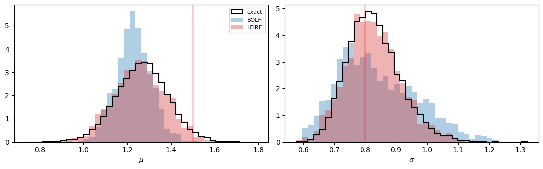
LFIRE reproduces the exact posterior most closely of the three methods here, without a hand-tuned distance or tolerance. It uses a similar number of simulations as rejection ABC, though: every log-ratio evaluation needs its own n_theta simulations. It pays off when good summaries are hard to combine by hand (many candidate summaries, L1 picks the useful ones) and when simulations at one \(\theta\) can be generated in parallel.

plot_lfire from psiphy.plotting.corner draws the grid posterior after lfire.posterior_grid() or lfire.run_grid().

---

6 Acquisition functions and batch proposals

acquisition chooses where to simulate next (all implemented in psiphy.utils.bayesian_opt):

Name	Picks points with	Behaviour
'LCB' (default)	low \(\mu - \kappa\sigma\)	explores in proportion to kappa (default 1.96)
'EI'	high expected improvement over the best \(\hat d\)	concentrates near the minimum; xi adds exploration
'PI'	high probability of improvement	most exploitative

batch_size=q proposes \(q\) points per round (kriging believer: each pick is added to the GP as a fake observation at its predicted mean, so the next pick goes elsewhere). The \(q\) simulations of a round are independent, so on a cluster they can run in parallel.

runs = {
    'LCB':                 dict(acquisition='LCB'),
    'EI':                  dict(acquisition='EI'),
    'LCB, batch_size = 5': dict(acquisition='LCB', batch_size=5),
}
fig, axes = plt.subplots(1, 3, figsize=(15, 4), sharex=True, sharey=True)
for ax, (name, kw) in zip(axes, runs.items()):
    batch = kw.pop('batch_size', 1)
    b = BOLFI(lambda t: discrepancy(gs.simulate(t)), prior, verbose=False, **kw)
    b.learn_likelihood(n_calls=60, batch_size=batch, random_state=1)
    s = b.sample_posterior(3000, method='MCMC', n_walkers=32, n_burn=500)
    ax.plot(*s_exact[::10].T, '.', c='0.75', ms=2)
    ax.scatter(*b.X.T, c=np.arange(len(b.X)), cmap='viridis', s=14, zorder=3)
    ax.plot(*theta_true, 'r*', ms=12)
    ax.set(title=f'{name}\nmean {np.round(s.mean(0), 2)}, std {np.round(s.std(0), 2)}', xlabel=labels[0])
axes[0].set_ylabel(labels[1])
plt.tight_layout()
plt.show()

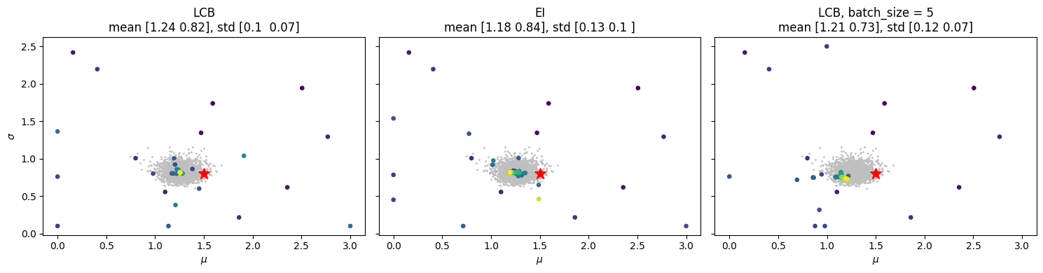
Colour shows the order of evaluation (dark = early). Grey: exact posterior samples.

---

7 Saving and resuming

With filename=, the evaluated points are stored after learning. A later call with the same file continues from them, adding n_calls new simulations — so the expensive part can be split across jobs.

fn = os.path.join(tempfile.mkdtemp(), 'bolfi.pkl')
b1 = BOLFI(lambda t: discrepancy(gs.simulate(t)), prior, verbose=False)
b1.learn_likelihood(n_calls=30, filename=fn, random_state=0)

b2 = BOLFI(lambda t: discrepancy(gs.simulate(t)), prior, verbose=False)
b2.learn_likelihood(n_calls=20, filename=fn, random_state=1)   # resumes from the 30 stored points
print('evaluations after resume:', len(b2.y))

evaluations after resume: 50

---

Summary

Task	Code
Rejection ABC	rABC(simulator, distance, x_obs, prior, bounds, N, eps).run()
LFIRE	LFIRE(simulator, x_obs, prior, summary=...), then learn_posterior(n_calls) or run_grid(n_grid)
BOLFI	BOLFI(distance_fn, prior, acquisition='LCB')
Learn	learn_likelihood(n_calls, batch_size=1, filename=None)
Sample	sample_posterior(n, method='MCMC' \| 'NestedSampling' \| 'IS' \| 'SMC')
Surrogate	log_likelihood(theta), predict_distance(theta, return_std=True)

BOLFI and LFIRE share sample_posterior, save_model / load_model (resumable learning) and batch_size. Options worth knowing: distance_kernel='exp' | 'gaussian' | callable (maps \(d\) to \(\log\mathcal{L}\)), learn_log_dist=True (model \(\log d\) when \(d\) spans orders of magnitude).