MCMC sampling and priors

This notebook covers the MCMC tools in psiphy.mcmc and the prior specifications in psiphy.utils.prior:

1. Priors: uniform, log-uniform, Gaussian and mixtures

2. Sampling a posterior with MHSampler (emcee backend)

3. Convergence diagnostics: traces, autocorrelation time, burn-in

4. Checking the result against the analytic posterior

5. Saving, reloading and extending a chain

6. Informative priors

The test problem is NoisyLine (a straight line with Gaussian noise). Its posterior is Gaussian with a closed form, so every result can be checked exactly.

Related notebooks: Nested sampling and evidence (posterior + Bayes factors), Importance sampling and SMC, Likelihood-free inference (simulator only).

import os
import tempfile

import numpy as np
import matplotlib.pyplot as plt

from psiphy.mcmc import MHSampler
from psiphy.utils.prior import UniformPrior, LogUniformPrior, GaussianPrior, MixturePrior
from psiphy.toy_models import NoisyLine
from psiphy.plotting.diagnostics import SampledDistribution, plot_triangle

np.random.seed(42)

---

1 Priors

Every prior in psiphy.utils.prior shares one interface, so the same object works with MCMC, nested sampling, importance sampling/SMC and BOLFI:

Method	Purpose
sample(n)	draws, shape (n, ndim)
log_prob(theta)	single point → float; batch (n, ndim) → (n,)
prior_transform(u)	unit cube → parameters (used by nested sampling)
to_scipy(), to_torch(), to_sbi()	conversion to other libraries

priors = {
    'Uniform(0, 10)':              UniformPrior([(0, 10)]),
    'LogUniform(0.1, 10)':         LogUniformPrior([(0.1, 10)]),
    'Gaussian(5, 1.5²)':           GaussianPrior([5.0], [1.5**2]),
    'Mixture: 0.3 N(2,.5²) + 0.7 N(7,1²)': MixturePrior(
        [GaussianPrior([2.0], [0.25]), GaussianPrior([7.0], [1.0])], weights=[0.3, 0.7]),
}

grid = np.linspace(0.01, 11, 500)[:, None]
fig, axes = plt.subplots(1, 4, figsize=(15, 3), sharey=False)
for ax, (name, p) in zip(axes, priors.items()):
    ax.hist(p.sample(20000)[:, 0], bins=60, range=(0, 11), density=True, alpha=0.5, label='samples')
    ax.plot(grid[:, 0], np.exp(p.log_prob(grid)), 'k', lw=1.5, label='exp(log_prob)')
    ax.set(title=name, xlabel=r'$\theta$')
axes[0].legend(fontsize=8)
plt.tight_layout()
plt.show()

Named bounds can be passed as a dict; the keys become prior.names and are picked up by the samplers. prior_transform maps uniform draws on \([0,1]^d\) to the prior, which is how nested samplers use it.

prior = UniformPrior({'slope': (-3, 3), 'intercept': (0, 10)})
print('names            :', prior.names)
print('log_prob (inside):', prior.log_prob([0.0, 5.0]))
print('log_prob (batch) :', prior.log_prob(np.array([[0.0, 5.0], [9.0, 5.0]])))
print('prior_transform  :', prior.prior_transform([0.5, 0.5]))

names            : ['slope', 'intercept']
log_prob (inside): -4.094344562222101
log_prob (batch) : [-4.09434456        -inf]
prior_transform  : [0. 5.]

---

2 Problem: fitting a noisy line

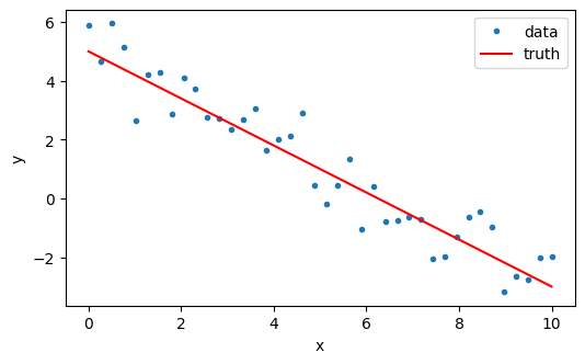
Data: \(y_i = m x_i + b + \varepsilon_i\) with \(\varepsilon_i \sim \mathcal{N}(0, \sigma^2)\) and known \(\sigma\). With a flat prior the posterior on \((m, b)\) is Gaussian with covariance \(\sigma^2 (A^\top A)^{-1}\), where \(A = [x, 1]\), centred on the least-squares fit.

line = NoisyLine(Nx=40, noise_sigma=0.8)
theta_true = np.array([-0.8, 5.0])
y_obs = line.simulate(theta_true)

def log_posterior(theta):
    lp = prior.log_prob(theta)
    return lp + line.log_prob(theta, y_obs) if np.isfinite(lp) else -np.inf

# analytic posterior (flat prior, posterior well inside the box)
A = np.column_stack([line.x, np.ones_like(line.x)])
post_cov = line.noise_sigma**2 * np.linalg.inv(A.T @ A)
post_mean = np.linalg.solve(A.T @ A, A.T @ y_obs)
print('analytic posterior mean:', post_mean.round(3))
print('analytic posterior std :', np.sqrt(np.diag(post_cov)).round(3))

plt.figure(figsize=(6, 3.5))
plt.plot(line.x, y_obs, '.', label='data')
plt.plot(line.x, theta_true[0] * line.x + theta_true[1], 'r-', label='truth')
plt.xlabel('x'); plt.ylabel('y'); plt.legend()
plt.show()

analytic posterior mean: [-0.816  5.188]
analytic posterior std : [0.043 0.248]

---

3 Running MHSampler

MHSampler wraps emcee.EnsembleSampler. Starting from a single point, the walkers are spread into a small Gaussian ball (init_scale, relative). Starting from prior draws, pass an array of shape (n_walkers, n_dim).

sampler = MHSampler(log_posterior, n_walkers=32, param_names=prior.names)
sampler.run(prior.sample(32), n_steps=3000, progress=False)

print('chain shape (steps, walkers, dim):', sampler.get_chain().shape)
print('mean acceptance fraction        :', sampler.acceptance_fraction.mean().round(3))

chain shape (steps, walkers, dim): (3000, 32, 2)
mean acceptance fraction        : 0.712

---

4 Convergence diagnostics

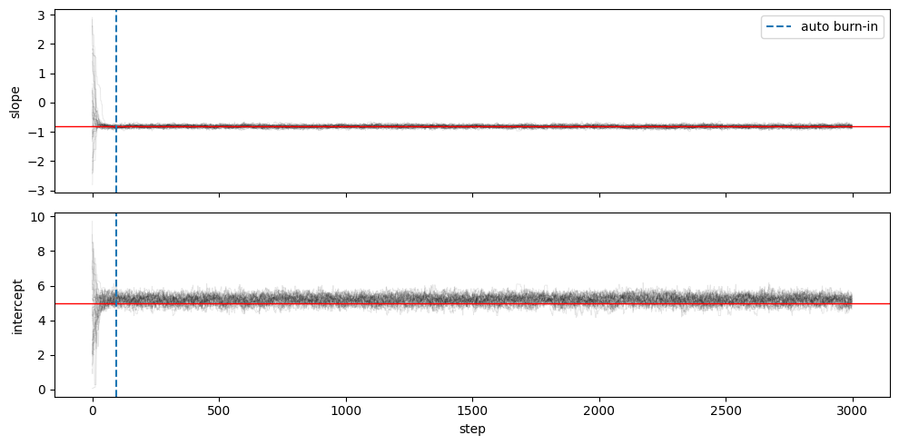
Walkers start spread over the whole prior and need some steps to reach the posterior. The integrated autocorrelation time \(\tau\) measures how many steps it takes for the chain to forget its state. Common practice: discard a few \(\tau\) as burn-in and run for at least ~50 \(\tau\). discard="auto" drops \(3\,\max(\tau)\) steps.

chain = sampler.get_chain()
tau = sampler.autocorr_time()
burn = int(3 * tau.max())
print('autocorrelation time:', tau.round(1), ' → auto burn-in =', burn, 'steps')

fig, axes = plt.subplots(2, 1, figsize=(10, 5), sharex=True)
for i, (ax, name) in enumerate(zip(axes, prior.names)):
    ax.plot(chain[:, :, i], 'k', alpha=0.1, lw=0.6)
    ax.axhline(theta_true[i], c='r', lw=1)
    ax.axvline(burn, c='C0', ls='--', label='auto burn-in')
    ax.set_ylabel(name)
axes[0].legend(loc='upper right')
axes[-1].set_xlabel('step')
plt.tight_layout()
plt.show()

autocorrelation time: [25.7 31.6]  → auto burn-in = 94 steps

---

5 Posterior and comparison with the analytic result

summary = sampler.summary(discard='auto')

     param        mean         std      median      tau
     slope     -0.8164     0.04297      -0.817     25.7
 intercept       5.184      0.2475       5.186     31.6
acceptance fraction = 0.712, n_samples = 92992

samples = sampler.get_chain(flat=True, discard='auto', thin=5)
print('MCMC mean :', samples.mean(0).round(3), '   analytic:', post_mean.round(3))
print('MCMC std  :', samples.std(0).round(3), '   analytic:', np.sqrt(np.diag(post_cov)).round(3))

fig = plot_triangle(samples, labels=['m', 'b'], true_values=theta_true, engine='corner',
                    bins=40, plot_datapoints=False, fill_contours=True, levels=(0.68, 0.95))
# overlay the analytic 1σ/2σ ellipse in the 2-D panel
ax = fig.axes[2]
vals, vecs = np.linalg.eigh(post_cov)
t = np.linspace(0, 2 * np.pi, 200)
for k in (1, 2):
    ell = post_mean[:, None] + vecs @ (k * np.sqrt(vals)[:, None] * np.vstack([np.cos(t), np.sin(t)]))
    ax.plot(*ell, 'C1--', lw=1)
fig.suptitle('MHSampler vs analytic posterior (orange dashed: 1σ, 2σ)', y=1.02)
plt.show()

MCMC mean : [-0.816  5.184]    analytic: [-0.816  5.188]
MCMC std  : [0.043 0.247]    analytic: [0.043 0.248]

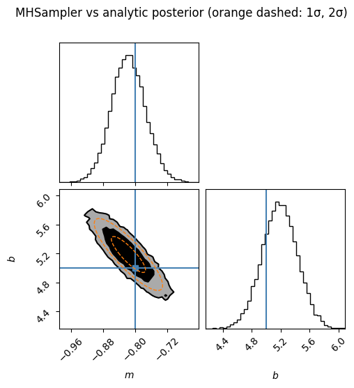
Why is :math:`b` not centred on the truth? The MCMC result matches the analytic posterior, and that posterior is centred on the least-squares fit to these 40 points. The noise in this particular data set moves that fit away from the true line by a fraction of a standard deviation (printed below). Every correct method follows the data; checking for bias requires many data sets — see Section 7 of the Importance sampling and SMC tutorial.

offset = (post_mean - theta_true) / np.sqrt(np.diag(post_cov))
print('least-squares fit:', post_mean.round(3), ' truth:', theta_true, ' offset (sigma):', offset.round(2))

least-squares fit: [-0.816  5.188]  truth: [-0.8  5. ]  offset (sigma): [-0.38  0.76]

The same samples plug straight into the diagnostics tools (see the Plotting diagnostics tutorial) for z-scores, credible intervals and comparisons.

dist = SampledDistribution(samples, true_values=theta_true, labels=['m', 'b'])
for name, ci in zip(prior.names, dist.credible_intervals(levels=(68, 95))):
    print(f"{name:10s} median={ci['median']:.3f}  68% [{ci['lo68']:.3f}, {ci['hi68']:.3f}]")
print('z-scores:', np.round(dist.z_scores(), 2))

slope      median=-0.817  68% [-0.859, -0.774]
intercept  median=5.185  68% [4.941, 5.429]
z-scores: [0.38 0.75]

---

6 Saving, reloading and extending a chain

Pass filename= to store the chain in HDF5 (needs h5py). The file can be reloaded, and run(n_steps=...) without a starting point continues from the last state — useful for long jobs on a cluster with wall-time limits.

tmpdir = tempfile.mkdtemp()
fn = os.path.join(tmpdir, 'line_chain.h5')

s1 = MHSampler(log_posterior, n_walkers=32, filename=fn)
s1.run(prior.sample(32), n_steps=500)
print('first job :', s1.n_steps, 'steps')

# later, e.g. in a new job:
s2 = MHSampler.load(fn, log_prob_fn=log_posterior)
s2.run(n_steps=1000)
print('after resume:', s2.n_steps, 'steps stored in', os.path.basename(fn))

first job : 500 steps
after resume: 1500 steps stored in line_chain.h5

---

7 Informative priors

Swapping the prior is a one-line change. A Gaussian prior on the intercept (say from an earlier measurement) tightens the intercept and, through the correlation, the slope.

prior_inf = GaussianPrior(mean=[0.0, 5.0], cov=[10.0**2, 0.15**2], names=['slope', 'intercept'])
log_post_inf = lambda t: prior_inf.log_prob(t) + line.log_prob(t, y_obs)

s_inf = MHSampler(log_post_inf, n_walkers=32).run(prior.sample(32), n_steps=3000)
samples_inf = s_inf.get_chain(flat=True, discard='auto', thin=5)

fig, axes = plt.subplots(1, 2, figsize=(10, 3.5))
for i, (ax, name) in enumerate(zip(axes, prior.names)):
    ax.hist(samples[:, i], bins=50, density=True, alpha=0.5, label='flat prior')
    ax.hist(samples_inf[:, i], bins=50, density=True, alpha=0.5, label='Gaussian prior on b')
    ax.axvline(theta_true[i], c='r')
    ax.set_xlabel(name)
axes[0].legend()
plt.tight_layout()
plt.show()
print('std flat       :', samples.std(0).round(3))
print('std informative:', samples_inf.std(0).round(3))

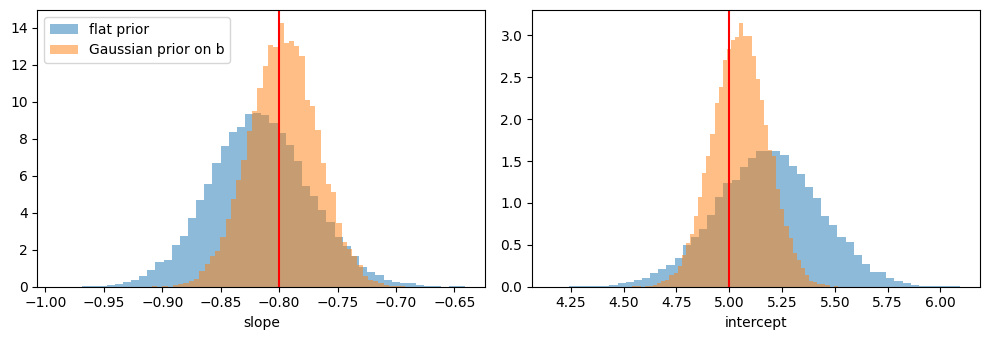
std flat       : [0.043 0.247]
std informative: [0.029 0.128]

---

Summary

Task	Code
Define a prior	UniformPrior({...}), LogUniformPrior, GaussianPrior, MixturePrior
Run MCMC	MHSampler(log_prob, n_walkers=32).run(theta_init, n_steps=...)
Diagnose	autocorr_time(), acceptance_fraction, trace of get_chain()
Samples	get_chain(flat=True, discard='auto', thin=...)
Summary	summary()
Checkpoint / resume	filename='chain.h5', MHSampler.load(...), run(n_steps=...)

Parallel evaluation: pass pool= (any object with a map method, e.g. a multiprocessing.Pool).