Nested sampling and Bayesian evidence

Nested sampling computes the Bayesian evidence (marginal likelihood)

\[\mathcal{Z} = \int \mathcal{L}(\theta)\, \pi(\theta)\, d\theta\]

and produces posterior samples as a by-product. The evidence is what MCMC does not give you: it is the quantity needed to compare models.

This notebook uses psiphy.mcmc.NestedSampler with the nautilus backend, which needs few likelihood calls (useful for expensive likelihoods) and can evaluate likelihoods in batches. The dynesty backend is a drop-in alternative if it is installed; the interface and the result format are identical:

NestedSampler(log_likelihood, prior, backend="dynesty")   # instead of "nautilus"

Contents:

1. Checking the evidence against an analytic value

2. Posterior samples and getdist export

3. Model comparison with Bayes factors

import numpy as np
import matplotlib.pyplot as plt
from getdist import plots

from psiphy.mcmc import NestedSampler
from psiphy.utils.prior import UniformPrior
from psiphy.toy_models import NoisyLine

np.random.seed(1)

---

1 Evidence of a Gaussian likelihood in a box

Take a normalised 2-D Gaussian likelihood and a uniform prior on a box much wider than the Gaussian. The integral of the likelihood is 1, and the prior density is \(1/V\), so \(\mathcal{Z} = 1/V\) exactly.

mean = np.array([0.5, -1.0])
cov = np.array([[1.0, 0.3], [0.3, 0.5]])
icov = np.linalg.inv(cov)
norm = -0.5 * np.log(np.linalg.det(2 * np.pi * cov))

def log_like_gauss(theta):
    d = theta - mean
    return norm - 0.5 * d @ icov @ d

box = UniformPrior({'x': (-10, 10), 'y': (-10, 10)})
ns = NestedSampler(log_like_gauss, box, backend='nautilus', n_live=500, seed=0)
res = ns.run(dlogz=0.01).get_result()

print(f"log Z (nautilus) = {res['log_evidence']:.3f}")
print(f"log Z (analytic) = {np.log(1 / 400):.3f}")
print(f"effective sample size = {res['ess']:.0f}")

log Z (nautilus) = -5.988
log Z (analytic) = -5.991
effective sample size = 10066

get_result() returns the same keys for every backend:

Key	Content
log_evidence, log_evidence_err	\(\log\mathcal{Z}\) and its error (None for nautilus)
samples, weights	weighted posterior samples (weights aligned with samples)
equal_weight_samples	resampled, unweighted draws
log_likelihood, ess, backend	per-sample log-likelihood, effective sample size, backend name

---

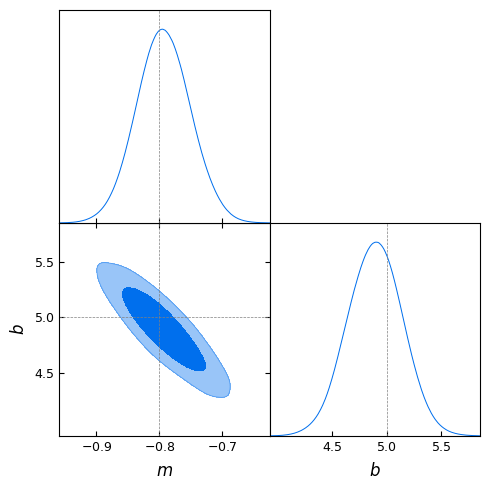
2 Posterior: fitting a noisy line

The likelihood function takes only theta; the data are captured in a closure. The prior object supplies the unit-cube transform and the parameter names.

line = NoisyLine(Nx=40, noise_sigma=0.8)
theta_true = np.array([-0.8, 5.0])
y_obs = line.simulate(theta_true)

prior_line = UniformPrior({'m': (-3, 3), 'b': (0, 10)})
ns_line = NestedSampler(lambda t: line.log_prob(t, y_obs), prior_line, backend='nautilus', seed=0)
res_line = ns_line.run().get_result()

post_mean = np.average(res_line['samples'], weights=res_line['weights'], axis=0)
print('posterior mean:', post_mean.round(3), '  truth:', theta_true)
print(f"log Z = {res_line['log_evidence']:.2f}")

posterior mean: [-0.793  4.893]   truth: [-0.8  5. ]
log Z = -53.90

mc = ns_line.to_getdist(labels=['m', 'b'], label='nautilus')
g = plots.get_subplot_plotter(width_inch=5)
g.triangle_plot(mc, filled=True, markers={'m': theta_true[0], 'b': theta_true[1]})
plt.show()

Removed no burn in

---

3 Model comparison: is there curvature?

Compare a straight line (\(M_1\): \(y = m x + b\)) with a quadratic (\(M_2\): \(y = a x^2 + m x + b\)). The Bayes factor

\[\ln B_{21} = \ln \mathcal{Z}_2 - \ln \mathcal{Z}_1\]

weighs goodness of fit against model complexity: the extra parameter \(a\) spreads prior mass over values the data don’t support, which is penalised (Occam’s razor). A rough guide (Jeffreys/Kass–Raftery): \(|\ln B| < 1\) inconclusive, \(1\)–\(3\) positive, \(3\)–\(5\) strong, \(>5\) very strong.

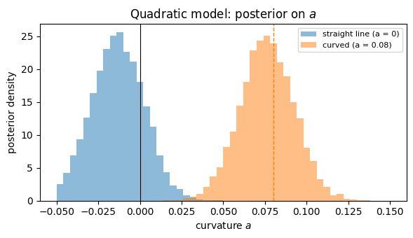
We test two data sets: one generated from a straight line and one with mild curvature.

x = line.x
sigma = line.noise_sigma

def make_loglike(y, model):
    def loglike(t):
        mu = model(t)
        return -0.5 * np.sum((y - mu) ** 2) / sigma**2 - 0.5 * len(y) * np.log(2 * np.pi * sigma**2)
    return loglike

linear = lambda t: t[0] * x + t[1]
quadratic = lambda t: t[0] * x**2 + t[1] * x + t[2]

prior_M1 = UniformPrior({'m': (-3, 3), 'b': (0, 10)})
prior_M2 = UniformPrior({'a': (-0.3, 0.3), 'm': (-3, 3), 'b': (0, 10)})

datasets = {
    'straight line (a = 0)':  -0.8 * x + 5.0 + np.random.normal(0, sigma, x.size),
    'curved (a = 0.08)':      0.08 * x**2 - 0.8 * x + 5.0 + np.random.normal(0, sigma, x.size),
}

rows = []
for name, y in datasets.items():
    r1 = NestedSampler(make_loglike(y, linear), prior_M1, backend='nautilus', seed=0).run().get_result()
    r2 = NestedSampler(make_loglike(y, quadratic), prior_M2, backend='nautilus', seed=0).run().get_result()
    rows.append((name, r1['log_evidence'], r2['log_evidence'], r2))

print(f"{'data':24s} {'ln Z (line)':>12s} {'ln Z (quad)':>12s} {'ln B_21':>9s}")
for name, z1, z2, _ in rows:
    print(f"{name:24s} {z1:12.2f} {z2:12.2f} {z2 - z1:9.2f}")

data                      ln Z (line)  ln Z (quad)   ln B_21
straight line (a = 0)          -52.46       -54.83     -2.37
curved (a = 0.08)              -55.96       -47.58      8.37

For straight-line data the Bayes factor favours the simpler model even though the quadratic fits at least as well; for curved data the quadratic wins clearly. The posterior on the curvature parameter shows why:

fig, ax = plt.subplots(figsize=(6, 3.5))
for (name, _, _, r2), c in zip(rows, ['C0', 'C1']):
    ax.hist(r2['samples'][:, 0], weights=r2['weights'], bins=50, range=(-0.05, 0.15),
            density=True, alpha=0.5, color=c, label=name)
ax.axvline(0, c='k', lw=0.8)
ax.axvline(0.08, c='C1', ls='--', lw=1)
ax.set(xlabel='curvature $a$', ylabel='posterior density', title='Quadratic model: posterior on $a$')
ax.legend(fontsize=8)
plt.tight_layout()
plt.show()

---

Summary

Task	Code
Run	NestedSampler(log_likelihood, prior, backend='nautilus').run(dlogz=...)
Results	get_result() → log_evidence, samples, weights, equal_weight_samples, …
Plot	to_getdist() → getdist MCSamples
Compare models	\(\ln B_{21} = \ln\mathcal{Z}_2 - \ln\mathcal{Z}_1\)
Other backend	backend='dynesty' (also gives log_evidence_err)

The likelihood must be normalised (include constants such as \(-\tfrac12 N \ln 2\pi\sigma^2\)) when evidences of models with different data normalisations are compared; constants common to all models cancel in the Bayes factor.

Parallel evaluation: pass pool= (any object with a map method, e.g. a multiprocessing.Pool).